B-trees : A Survey
B-trees are the fascinating data structures at the heart of almost every piece of data storage and retrieval technology you've ever dealt with. Ever created a relational database table with an indexed column? B-trees. Ever accessed a file in a filesystem? B-trees.
They are so useful because they:
- Keep keys sorted, no matter what order they are inserted
- Build up wide but shallow trees to traverse
- Work well with external index storage (i.e. disks)
How They Work, A Love Letter In Pictures
To illustrate how B-trees work, I'm going to use pictures. Later we can get into the code. To make the pictures intelligible, we're going to have to use a smaller degree; each node in our B-tree will only be able to hold 5 keys and 6 links.
We're also going to skip some of the boring parts and start out at "step 1" with 4 elements already inserted into our B-tree:
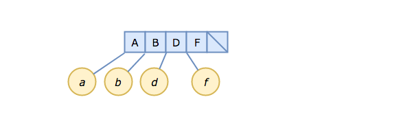
The blue boxes are the slots in the B-tree node, each containing a key. There are pointers on each side of each slot. For leaf nodes (and our root node is a leaf node at this point), those pointers point to the actual data being stored for each key, i.e., A → a, B → b, etc.
Now, let's insert a new key/value pair, E → e.
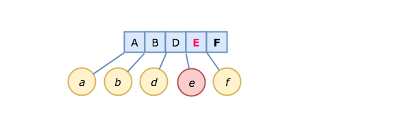
Both F and f get moved to make room for E → e in the correct (sorted) position.
This is the killer feature of B-trees; as elements are inserted, keys remain in sort order. This is why databases and filesystems make such extensive use of them.
We could just stop here, and wait for the next insertion, but we're going to do some proactive housekeeping first. Our B-tree node is now full. We need to grow the tree to give ourselves some breathing room.
We'll do this by splitting our node in two, right down the middle, at D, and migrating D "up" to become the new root. To the left we will place keys A and B (which are strictly less than D), and to the right, E and F.
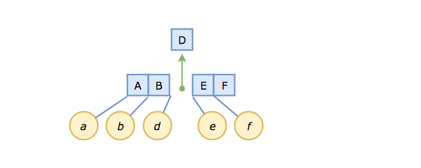
The choice of D is important. We're hedging our bets by picking the median, because that gives equal footing when key/value pairs are inserted in random order.
Our B-tree now spans three nodes, and looks like this:
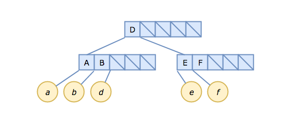
Note, particularly, that it is the pointer after B that points to d. You can (and should!) think of this as the pointer between B and D — viewed that way, it's no different from the structure we had in steps 1 and 2.
Now we are starting to see the tree structure emerge.
What happens if we insert C → c?
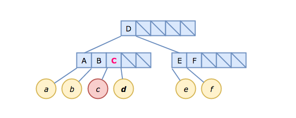
Insertion starts by considering the root node, which just contains D. Since C < D, and the root node is not a leaf node, we follow the pointer link to the left of D and arrive at the leftmost child node [A, B]. This is a leaf node, so we insert C → c right after B, remembering to shift the link to d one slot to the right (D > C, after all). This does not fill the child node, so we are done.
On The Importance of Being Proactive
Above, we split the node as soon as it was full.
We didn't have to. We could just as easily have waited until the next insertion, and split the node then, to make room for our new key/value. That would lead to more compact trees, at the expense of a more complicated implementation.
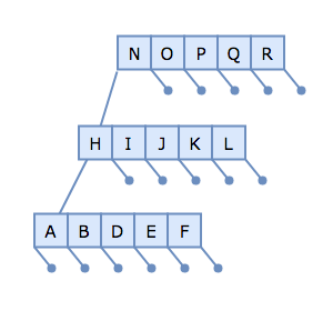
To understand why, let's consider a pathological case where we have several full B-tree nodes along a single ancestry line:
Then, let's try to insert the key/value pair C → c. To do so, we traverse the root node to the H-node, to the A-node. Since the A-node is full, we need to split it at the median, D:
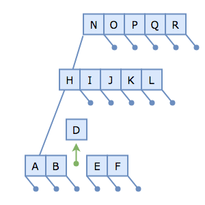
Uh-oh. We have nowhere to put D. Normally, it would migrate up the tree and be inserted into the H-node, but the H-node is full!
We could split the H-node, but it suffers the same problem; its parent (the N-node) is also full! Our simple insertion has cascaded into a sequence of partitioning operations:
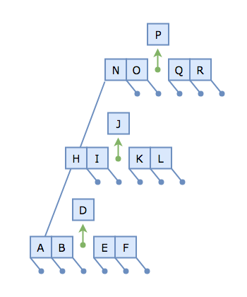
Being proactive, and splitting on the way down (as the literature puts it), means that we can never get into this problematic scenario in the first place.
In Algorithms (1983), Sedgewick has this to say:
As with top-down 2-3-4 trees, it is necessary to "split" nodes that are "full" on the way down the tree; any time we see a k-node attached to an M node, we replace it by a (k + 1)-node attached to two M/2 nodes. This guarantees that when the bottom is reached there is room to insert the new node.
Aside: Algorithms is a wonderful text, worthy of study. Don't let anyone tell you that seminal computer science texts from the 80's (or before!) are obsolete.
By taking this advice one step further, and splitting on insertion, we can ensure that traversal / retrieval doesn't need to be bothered with such trifles.
Some Mathematics To Consider
I spent a fair amount of time studying B-trees for a project of mine, focusing mainly on how best to size the B-tree node for optimal density and tree height.
Tree height is important because our data values are only stored in the leaf nodes. Therefore, every single lookup has to traverse the height of the tree, period. The shorter the tree, the fewer nodes we have to examine to find what we want.
Given that most B-trees live on-disk, with only the root node kept in memory, tree height becomes even more important; fewer disk accesses = faster lookup.
The following equations consider B-trees of degree \(m\) (for maximum number of children allowed in a node).
First, we need to figure out the minimum number of keys required of interior nodes, which we'll call \(d\). Usually, this is:
$$d = ⌈{m/2}⌉$$
Using a median-split, we should never have fewer than \(d\) keys per interior node. The root node is special, since we have to start somewhere, and the leaf nodes are likewise exempt.
The worst-case height then, given \(n\) items inserted, is:
$$h_{worst} ≤ ⌊{log_d({n + 1}/2)}⌋$$
and the best-case height is:
$$h_{best} = ⌈{log_m({n + 1})}⌉ - 1$$
Common wisdom has it that you should choose a natural block size as your node size, in octets. That's either 4096 bytes (4k) or 8192 bytes (8k), so let's run through the calculations.
For \(T = 4096\):
$$m = 340$$
$$d = ⌈m/2⌉ = ⌈340/2⌉ = ⌈170⌉ = 170$$
We can fit 170 pointers and 169 keys per B-tree node. Our worst-case height, given minimal node usage is:
$$h_{worst} ≤ ⌊{log_d({n + 1}/2)}⌋$$
For my analysis, I was trying to find best- and worst-case scenarios given \(2^32 - 1\) items (one for every second I could fit in a 32-bit unsigned integer). \(n + 1\) then simplifies to just \(2^32\), and dividing by two knocks one off of the exponent, leaving \({n+1}/2 = 2^31\):
$$h_{worst} ≤ ⌊{log_170({2^31)}⌋ ≤ ⌊{3.675}⌋ ≤ 3$$
So with minimally dense nodes, we can expect to traverse 3 nodes to find a value corresponding to any given key. Let's see about best-case scenario. As before, \(n + 1\) simplifies down to \(2^32\):
$$h_{best} = ⌈{log_m({n + 1})}⌉ - 1$$
$$h_{best} = ⌈{log_340({2^32)}⌉ - 1 = ⌈3.805⌉ - 1 = 3$$
So, 3, again. That's what I call balance.
For \(T = 8192\):
$$m = 681$$
$$d = ⌈m/2⌉ = ⌈681/2⌉ = ⌈340.5⌉ = 341$$
Using \({n+1}/2 = 2^31\), as before, we can calculate the worst-case for an 8k-page B-tree:
$$h_{worst} ≤ ⌊{log_d({n + 1}/2)}⌋$$
$$h_{worst} ≤ ⌊{log_341({2^31)}⌋ ≤ ⌊{3.684}⌋ ≤ 3$$
As with 4k pages, we can expect to look at 3 nodes before we find the value we seek. Not bad.
What about \(h_{best}\)?
$$h_{best} = ⌈{log_m({n + 1})}⌉ - 1$$
$$h_{best}= ⌈{log_681({2^32)}⌉ - 1 = ⌈3.4⌉ - 1 = 3$$
It would seem that a choice between 4k and 8k won't affect our best and worst case heights; they are always 3.
The Literature
If you're interested in the genesis of B-trees, you'll want to read Bayer and McCreight's 1970 paper Organization and Maintenance of Large Ordered Indices.
Douglas Comer's 1979 review / survey of B-trees, The Ubiquitous B-Tree, covers the basics of B-trees, explains their ascent to ubiquity, and discusses several major variations, like B+-trees, and their relative merits.
Happy Hacking!

James works on the Internet, spends his weekends developing new and interesting bits of software and his nights trying to make sense of research papers.
Currently exploring just how much data you can shove though DuckDB before it explodes.